Mt. Eden Computer Applications I Class

Excel YOYO: PART 1 Commission

Click here for the file that you need:

Commission.xlsx

In the Commission.xlsx file:

1. Click cell E3.
   
   
2. Type: =SUM(B3:D3).
   
   
3. Press Enter (the return key).
   
   
4. Press the up arrow, cell E3 should be selected.
   Notice the formula appears in the Formula Bar.
   
   
5. Click the Copy button in the Tool Bar.
   
   
6. Select cells E4 through E8
   
   
7. Click Paste .
   
   
8. In cell F3, type: =E3*.06
   
   
9. Press Enter.
   
   
10. Press the up arrow, cell E3 should be selected.
    Notice the formula appears in the Formula Bar.
    
    
11. Copy or distribute the formula into cells F4 through F8.
    
    
12. Select cell F10.
    
    
13. Click the AutoSum drop-down arrow and select Count Numbers.
    
    
14. Select cells F3:F8.
    
    
15. Press Enter.
    
    
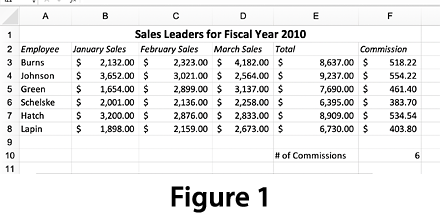
16. Your document should look like
    Figure 1 ==>
    
    
17. Select the cell range A2:B8.
    
    
18. In the Insert tab of the ribbon, click on the Column button and choose 2-D Clustered Column.
    
    
19. With the chart still selected, go to the Chart Design tab of the ribbon,
    click on the Add Chart Element button Axis Titles>Primary Horizontal Axis.
    
    
20. Type Employees.
    
    
21. Click again on the Add Chart Element button and select
    Axis Titles>Primary Vertical Axis.
    
    
22. Type: Sales (in Dollars).
    
    
23. Select the chart title, January Sales, and make it bold and 18points.
    
    
24. Feel free to set a Chart Style and other features to the chart.
    
    
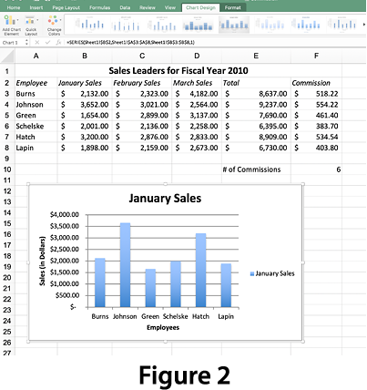
25. Move the chart and use the sizing handles to adjust the chart size to fit in the window below the data in the worksheet.
    See Figure 2 ==>
    
    
26. Done.

SAVE YOUR DOCUMENT.

TURN IN YOUR DOCUMENT.

Go to PART 2...